1 - Plotting multiple histograms on the same graph

Recently, while trying to compare the distribution of two samples, I discovered that you can plot both on the same graph in base R, which is a nice feature if you just want to examine the data quickly. We can explore this with a psychological dataset from the Open Psychometrics site. This hosts a range of open psychometric tests and stores the data in an accessible form. Let’s pull out the data for the Rosenberg Self-Esteem Scale (note that there are two different scoring methods in common use on this scale - on the website they have used a 1 - 4 Likert scale for the data output as a csv, but it is not unusual to see the use of a 0 - 3 scale, (which is the method used to give participants on the website feedback) so we need to be cautious when comparing these total scores with published norms - see https://socy.umd.edu/about-us/using-rosenberg-self-esteem-scale.

First we will load two packages we are going to use. We want the tidyverse for manipulating the variables and we will use the psych package for creating total scores on the measure itself.

library(tidyverse)
library(psych)

Next we want to set an url object to direct the download.file() to the right place to pull the data. I have called it my_url for simplicity. We pass this as the first argument in the download.file() function. We then set a destination for the file to be saved with the dest argument. Finally we use unzip to unpack the zipped file.

my_url <- "http://openpsychometrics.org/_rawdata/RSE.zip"
download.file(url = my_url, dest="data.zip", mode="wb") 
unzip ("data.zip", exdir = "./")

Now we can import the data with the read_tsv() function. We can’t use the read_csv() function with the data, because despite having a .csv extension, the data is actually tab-separated not comma-separated.

df <- read_tsv("RSE/data.csv")

In the Rosenberg Self-Esteem scale Items 2, 5, 6, 8, 9 are normally reverse scored. However, whoever loaded the questions on the website put them in a different order, with items 3, 5, 8, 9, 10 needing reversing. We need to create a total score for the measure and to be mindful of the reverse coded items. The psych package provides a function for this called scoreFast. We need to pass it a list called keys.list which specifies the direction of each item in turn (items are scored as-is if they have no leading ‘-’ minus sign, but all items with a minus are reverse scored). We won’t bother recoding the data from the 1 - 4 scale to 0 - 3 as it makes little difference for your graphs.

keys.list <- list(c('Q1', 'Q2', '-Q3', 'Q4', '-Q5', 'Q6', 'Q7', '-Q8', '-Q9', '-Q10'))
df$total <- scoreFast(keys.list, items = df[1:10], totals = TRUE, min = 1, max = 4)

Now we have our dataset, we can look at comparing distributions. We might want to know if the distribution of self-esteem scores differs between men and women. Checking the codebook on the website, we can see that males are coded as ‘1’ and females as ‘2’.

men <- df %>% 
  filter(gender == 1)
women <- df %>% 
  filter(gender == 2)

So let’s plot the total self-esteem scores for the women in the sample as a simple histogram.

hist(women$total)

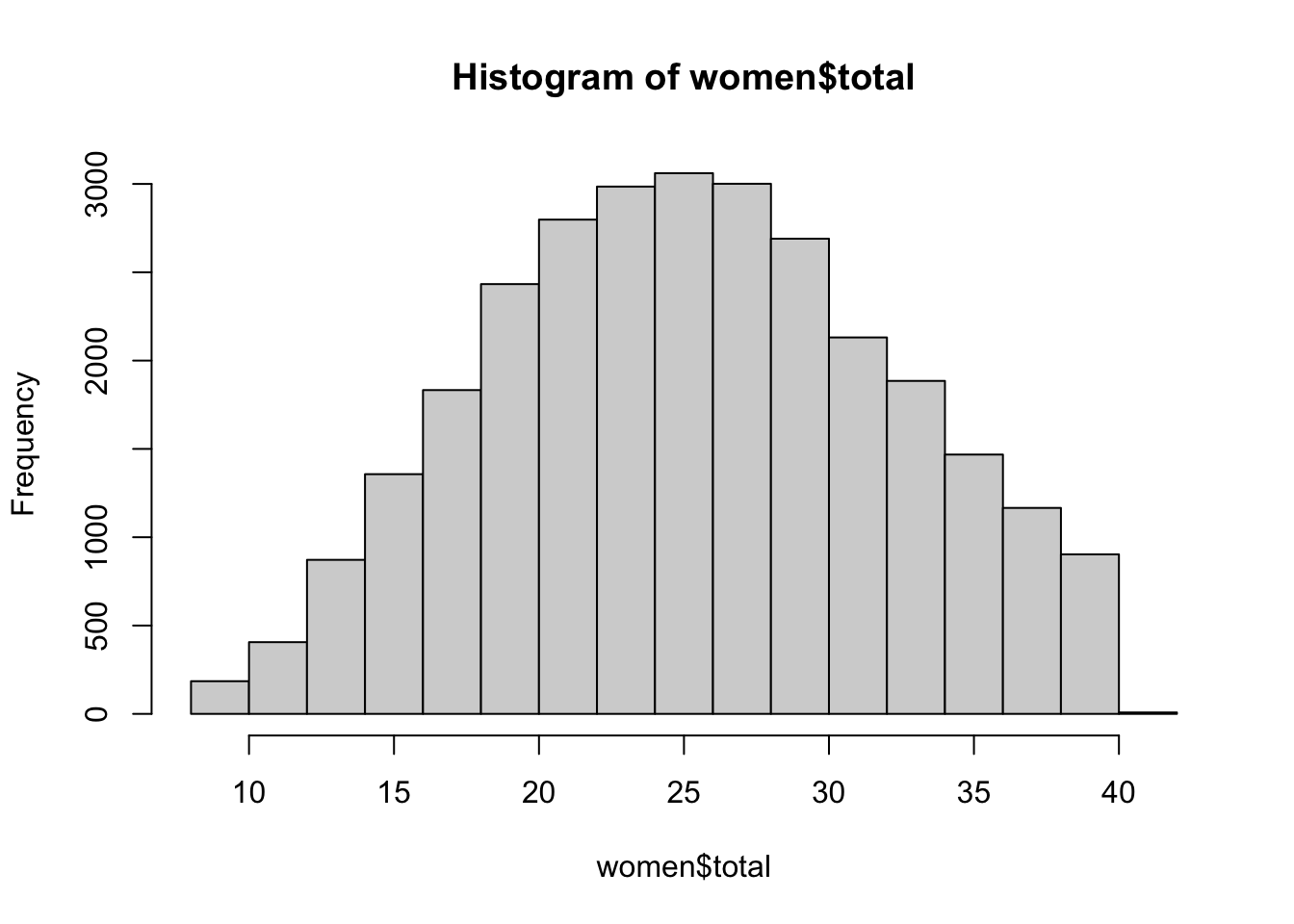We can see a fairly normal distribution of scores. We can check the mean, but we might predict it is around 25.

mean(women$total)

## [1] 25.74368

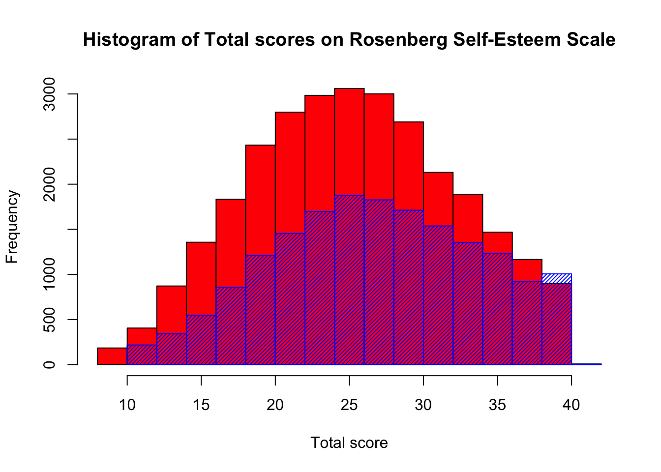
Next we can add the men’s scores to the same plot. Here we simply create the first plot, then make a second plot with the argument add set to TRUE. We will set the density to 35 so we can see through the bars on the histogram.

hist(women$total, col = 'red', main = "Histogram of Total scores on Rosenberg Self-Esteem Scale", xlab = "Total score")
hist(men$total, add = TRUE, col = 'blue', density = 35)

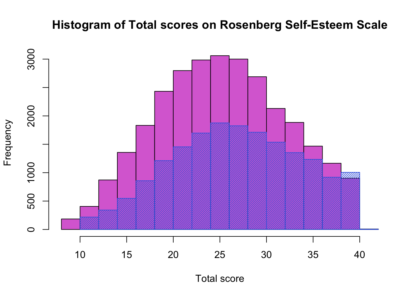
I have used the pipe to separate my data into individual gender dataframes, but this is only one way to do it, and I do find this code very easy to read. However, we could have done the same thing using a traditional R approach of indexing instead.

hist(df$total[df$gender== 2], col = 'orchid', main = "Histogram of Total scores on Rosenberg Self-Esteem Scale", xlab = "Total score")
hist(df$total[df$gender==1], add = TRUE, col = 'royalblue', density = 40)

Now we have seen the distributions, we might wonder if the sexes differ on the measure of self-esteem. Let’s run a quick t-test to see.

t.test(men$total, women$total)

## 
## 	Welch Two Sample t-test
## 
## data:  men$total and women$total
## t = 23.785, df = 37496, p-value < 2.2e-16
## alternative hypothesis: true difference in means is not equal to 0
## 95 percent confidence interval:
##  1.436304 1.694284
## sample estimates:
## mean of x mean of y 
##  27.30897  25.74368

Yes they do! With men having a significantly higher mean score on self-esteem (though the absolute difference is quite small.)