In the previous post on ‘pulling text data from the internet’, I experimented with pulling out the dream text from a sample of dreams from the website “DreamBank” at: http://www.dreambank.net/random_sample.cgi.

In this follow-up post, I will demonstrate some of the methods presented in Julia Silge and David Robinson’s book ‘Text Mining with R’ for processing text data, as applied to 400 dreams sampled from 4 collections in the dreambank. I used the methods described in the last post to pull out a random sample of 100 dreams from each of the following 4 groups:

• college_women (this was the sample used last time)
• hall_female
• hall_male
• vietnam_vet

The first set of dreams were recorded by college women by Calvin Hall from undergraduates in a course on personality at Western Reserve University in 1947 and 1948.

The second and third samples are also dreams collected by Calvin Hall and Robert L. Van de Castle, on which they based female and male norms in their book The Content Analysis of Dreams.

The sample listed as vietnam_vet are from the dreams of an American veteran of the Vietnam war, who suffered PTSD. The website has over 400 of his dreams which he donated from records he kept not long after returning from Vietnam.

Let’s begin by loading the three packages we are likely to use.

library(tidyverse)
library(tidytext)
library(stringr)

If you want to follow along with this post, the dataset I am about to load is “dream_df.csv”, which can be found on my github page: https://github.com/Christian-Ryan/netsite/tree/master/public/post

df <- read_csv("dreams_df.csv")
df <- df[,2:3]
df$sample <- as.factor(df$sample)

After sampling the four dream sets, using the techniques described in the last post, we now have a dataframe called df with two variables - sample and dream. We will use our custom_view() function we created last time to display snippets of dreams neatly formatted. We can also use the some() function from the car package to take a quick look at a selection of dreams across the dataframe. The some() function is very like head() and tail(), but has the advantage of returning a selection across the dataset, which allows us to see examples from each of the samples simultaneously.

custom_view <- function(x) data.frame(lapply(x, substr, 1, 56))
car::some(df) %>%
  custom_view()

##           sample                                                    dream
## 1  college_women I dreamed that I was in one of my classes and we had jus
## 2  college_women I dreamed I was in N__ Y__ with my family. We were out a
## 3  college_women I dreamt that our cleanlng woman, about 50, who has come
## 4    vietnam_vet I'm on the second floor of a mail fulfillment center, wa
## 5      hall_male I was in a big building in which a lot of people lived. 
## 6    hall_female I was working in a jewelry store. A man whom I knew in h
## 7    hall_female I was skating on the outdoor ice pond that used to be ac
## 8    hall_female I dreamed that I was driving along the street and the tr
## 9    hall_female Several people were telling me of somebody's death. Evid
## 10   hall_female I was at a summer resort. As I was going down the stairs

Julia Silge and David Robinson’s book Text Mining with R - A tidy approach sets off at a cracking pace, at least for relatively newbies to R such as myself. They assumes a degree of familiarity with tidyverse concepts and when they introduce concepts such as tidytext format, they can sometimes address three or four steps in one example. I will unpack some of these as individual steps to illustrate what is going on, while using our dream data as the material for processing.

At the moment our df only contains the sample name (a categorical variable with four values) and the text of the dream. It might be helpful to index the dreams before we tokenise the text in them. So let’s introduce a new variable that we will call dream_number. This will index each dream between 1 - 400 in the dataframe.

df <-  df %>%
  mutate(dream_number = row_number())

Now we have the dream_number variable added, we can unnest the tokens (split the text variable into individual words). The syntax for the unnest_tokens() function is to pipe in the dataframe (df), then supply the name of the variable to be created (word), followed by the variable containing the text we are going to tokenise - in this case “dream”.

df_word <- df %>%
  unnest_tokens(word, dream)
head(df_word)

## # A tibble: 6 × 3
##   sample        dream_number word   
##   <fct>                <int> <chr>  
## 1 college_women            1 i      
## 2 college_women            1 dreamed
## 3 college_women            1 that   
## 4 college_women            1 i      
## 5 college_women            1 was    
## 6 college_women            1 in

See that the word variable has replaced our dream variable and now each word is on a separate row - this is the tidytext format. unnest_tokens() has kept the variables sample and dream_number - it only transforms the input variable (dream) into the output variable (word). Notice also that the function has transformed into lower-case all the words in the word variable.

Tokenisation and N-Grams

It should be noted that when we use unnest_tokens() we are using a range of default values. We could have specified something other than single words in our output. The default value of the token argument is ‘word’. We can change this to ‘ngram’ and use an ‘n=’ to specify how many words should be kept as a group. Let us try a quick run with 3-word tokens instead of single words to demonstrate this behaviour.

df_trigrams <- df %>%
  unnest_tokens(trigrams, dream, token = "ngrams", n = 3)
head(df_trigrams)

## # A tibble: 6 × 3
##   sample        dream_number trigrams      
##   <fct>                <int> <chr>         
## 1 college_women            1 i dreamed that
## 2 college_women            1 dreamed that i
## 3 college_women            1 that i was    
## 4 college_women            1 i was in      
## 5 college_women            1 was in the    
## 6 college_women            1 in the office

So here we have set our output variable to ‘trigrams’ and specified the token argument to be equal to ‘ngrams’, and we have saved this as a new dataframe called ‘df_trigrams’. That gives us a better sense of the nature of the text. We can also run a count on this after grouping by sample.

df_trigrams %>%
  group_by(sample) %>%
  count(trigrams, sort = TRUE) %>%
  ungroup()

## # A tibble: 50,935 × 3
##    sample        trigrams              n
##    <fct>         <chr>             <int>
##  1 vietnam_vet   i tell him           33
##  2 hall_female   i was in             29
##  3 college_women i was in             25
##  4 vietnam_vet   the scene changes    23
##  5 college_women and i was            22
##  6 hall_female   seemed to be         19
##  7 college_women that i was           18
##  8 hall_female   that i was           17
##  9 hall_male     seemed to be         17
## 10 hall_female   and i was            16
## # … with 50,925 more rows

Here we can see that in the Vietnam veteran dream sample, the most common three word phrase was “I tell him”, whereas for the Hall Female and College Women the most common phrase was “I was in”. Using ngrams (units larger than one word), can be useful in exploring most frequently occurring phrases. It is notable that the phrase for the Vietnam vet was in the present tense, giving a sense of the immediacy and immersion of the dream experience, whereas those most frequent phrases of the other samples are in the past tense.

Single words (Bag of words approach)

We have not removed stop-words yet as this would undermine our exploration of ngrams. But this is the next step for our df_word dataset. The anti_join() function, takes two dataframes and keeps only those words that don’t occur in both dataframes. So this forms a convenient and easy way to filter out unwanted stopwords.

df_word <- df_word %>%
  anti_join(stop_words)

Then we can count the words and sort them into descending order.

df_word %>%
  count(word, sort = TRUE)

## # A tibble: 5,331 × 2
##    word         n
##    <chr>    <int>
##  1 house      133
##  2 dream      132
##  3 remember   125
##  4 car        118
##  5 people     110
##  6 girl       108
##  7 friend     101
##  8 time        95
##  9 woman       93
## 10 mother      85
## # … with 5,321 more rows

But before we create some plots of these words, we should check for any anomalies in the word variable of df_word. The sorted count is likely to give back expected results (high frequency genuine words). But there can be other text elements that we may want to filter out. This will become obvious if we count, but don’t sort.

df_word %>%
  count(word)

## # A tibble: 5,331 × 2
##    word       n
##    <chr>  <int>
##  1 ___        1
##  2 ______     1
##  3 00         2
##  4 1          4
##  5 1,500      1
##  6 10        13
##  7 100        3
##  8 105        1
##  9 107th      1
## 10 109        1
## # … with 5,321 more rows

The word variable contains some text elements that we would not regard as words. Let’s check where the underscores came from. To do this we must go back to our original (untokenised) dataset df, as we want to see the underscores in the context of the dream. We can use the str_which() function to identify which dreams contain underscores, matched to the pattern '___'. Then we can use this as an index on the df$dream variable, so that it just returns the context of the dreams with underscores. As there are three dreams with underscores, we will store this sequence of dreams and then take a look at the first one.

underscores <- df$dream[str_which(df$dream, pattern = "___")]
underscores[1]

## [1] "I dreamed about a young married couple whom I have known for a long time. They came to see us at our home. Although the home was ours, it resembled my Uncle's home in C___ and yet the dream seemed to take place in C ___.. They drove up in a Model A Ford & parked it in the front yard. We were in the living room talking when another Model A Ford drove up & in it were my sister & a friend of mine. I went out in the front yard, got in this couple's car, and started to talk to my sister. D___ my sister, asked me if I wanted to go to a play with J. She said that she and her husband weren't going. I realized that I would have to go with him alone, so I refused. Then they drove away and the wife came out in the yard. She seemed perturbed at my getting into their car, so she got into the car and backed it away. The car then suddenly changed into an old-fashioned bicycle. It was at this time that I felt antagonistic towards this couple."

So the pattern here seems to be that underscores are used to disguise the identity of named people in the dreams. We can choose to filter these out as they are not relevant to our analysis. But before we do this filtering, let’s also consider the numbers in the word variable column - again in a bag-of-words approach one could argue that these are not words and so are irrelevant. We want to create a pattern that identifies both digits and underscores, and then use a function to transform our word variable in the df_word dataframe.

Create pattern to remove numbers and underscores

We can use the function str_subset() to identify the elements of the word variable that we wish to remove. Let’s create a pattern that deals initially with the underscores and try str_subset() with it. The ‘+’ is not strictly necessary here, but it illustrates that we can identify at least one underscore by this combination.

str_subset(df_word$word, pattern = '_+')

##  [1] "n__"    "y__"    "c___"   "___"    "d___"   "h___"   "a___"   "a___"  
##  [9] "h__"    "______"

This has found ten instances of the underscore in the word variable. Now we want to find all the digits. We could use the regex shorthand [\d] or [:digit:]. Let’s use the latter first with str_subset to check it works.

str_subset(df_word$word, pattern = '[:digit:]')

##   [1] "169"    "80"     "90"     "30"     "60"     "40"     "45"     "4"     
##   [9] "20"     "4"      "5"      "2"      "34"     "34"     "309"    "219"   
##  [17] "6"      "5.00"   "8"      "5"      "45"     "20"     "45"     "22"    
##  [25] "50"     "23"     "45"     "22"     "30"     "45"     "22"     "11"    
##  [33] "8"      "8"      "12"     "3rd"    "26"     "20"     "20"     "22"    
##  [41] "60"     "70"     "20"     "25"     "20"     "27"     "23"     "52"    
##  [49] "23"     "7"      "30"     "2nd"    "2nd"    "7"      "10"     "10"    
##  [57] "2"      "1"      "1"      "2"      "999"    "e1"     "10"     "2"     
##  [65] "4"      "2"      "2"      "2"      "25"     "20"     "5"      "22"    
##  [73] "20"     "8"      "30"     "6"      "8"      "30"     "8"      "30"    
##  [81] "50"     "4"      "35"     "4"      "00"     "40"     "20"     "5"     
##  [89] "10"     "2"      "80"     "45"     "48"     "55"     "22"     "40"    
##  [97] "1992"   "200"    "300"    "100"    "20s"    "30s"    "1950s"  "2001"  
## [105] "2012"   "10"     "12"     "1990s"  "50s"    "1972"   "1950s"  "800"   
## [113] "45"     "60s"    "1970"   "45"     "1960s"  "105"    "1st"    "109"   
## [121] "110"    "116"    "121"    "122"    "2001"   "2012"   "138"    "139"   
## [129] "152"    "m16"    "m60"    "59"     "2001"   "2012"   "39"     "244"   
## [137] "1200"   "207"    "208"    "209"    "211"    "214"    "215"    "216"   
## [145] "800"    "411"    "42nd"   "217"    "218"    "219"    "2am"    "123"   
## [153] "220"    "1950s"  "2"      "20"     "20"     "19"     "20"     "22"    
## [161] "8"      "27"     "3"      "1,500"  "50"     "17"     "26"     "30"    
## [169] "10"     "70"     "6"      "3"      "4"      "30"     "33"     "45"    
## [177] "4"      "12"     "12"     "160"    "10"     "11"     "85"     "22"    
## [185] "11"     "10"     "50"     "300"    "30"     "10"     "20"     "440"   
## [193] "880"    "10"     "20"     "30"     "3000"   "3"      "3"      "3"     
## [201] "11"     "12"     "12"     "2"      "13"     "26"     "8"      "30"    
## [209] "11"     "30"     "19"     "7"      "30"     "8"      "30"     "28"    
## [217] "50"     "30"     "18"     "18"     "15"     "20"     "21"     "20"    
## [225] "6"      "30"     "19"     "16"     "2"      "23"     "25"     "35"    
## [233] "40"     "25"     "5"      "3"      "2"      "23"     "50"     "3"     
## [241] "3"      "1"      "2"      "2"      "23"     "40"     "35"     "8"     
## [249] "8"      "2"      "107th"  "16"     "27"     "10"     "8"      "60"    
## [257] "21"     "20"     "50"     "2"      "11"     "15"     "11"     "17"    
## [265] "17"     "2"      "34"     "45"     "49"     "52"     "55"     "3"     
## [273] "5"      "20"     "26"     "75.00"  "2"      "6"      "27"     "3"     
## [281] "4"      "00"     "1st"    "2nd"    "3rd"    "10"     "20"     "10"    
## [289] "30"     "50"     "50"     "11,000" "1"      "48th"   "4"      "6"     
## [297] "25th"   "100"    "100"

This works very nicely as well. However, to use these patterns with the tidyverse pipe, it is easier to use the fitler() function rather than str_subset(), and since it is convenient to chain steps in the pipe, we can use two calls to filter(), first by underscores and secondly by digits. And as we don’t want either of these in our dataset, we will set the “negate” argument to TRUE in both cases. An alternative method to delete the digits would be to use the capital “D” in the regex, but this way keeps our filters more uniform, both with a “negate = TRUE” argument.

df_word %>%
  filter(str_detect(word, pattern = "_", negate = TRUE)) %>%
  filter(str_detect(word, pattern = '[\\d]', negate = TRUE))

## # A tibble: 17,953 × 3
##    sample        dream_number word      
##    <fct>                <int> <chr>     
##  1 college_women            1 dreamed   
##  2 college_women            1 office    
##  3 college_women            1 directress
##  4 college_women            1 nurses    
##  5 college_women            1 nursing   
##  6 college_women            1 school    
##  7 college_women            1 forty     
##  8 college_women            1 told      
##  9 college_women            1 results   
## 10 college_women            1 i.q       
## # … with 17,943 more rows

Plot word frequencies

Now we have done some tidying on the dataset, we can plot the word frequencies - a simple way is to pass them through a filter so we only retain those words with a frequency greater than say n = 60. Notice we use mutate to create the new variables for the plot word (in the order of frequency) and n. We then filter by frequency, and pass the two new variables to the ggplot function. We also have to switch syntax at this point from the pipe ( %>% ) to the + sign between the layers of the ggplot() function. We flip the coordinates, as it allows us to keep the words in the horizontal aspect and makes it the plot easier to read.

df_word %>%
  count(word, sort = TRUE) %>%
  mutate(word = reorder(word, n)) %>%
  filter(n > 60) %>%
  ggplot(aes(x = word, y = n)) +
  geom_col()+
  coord_flip()

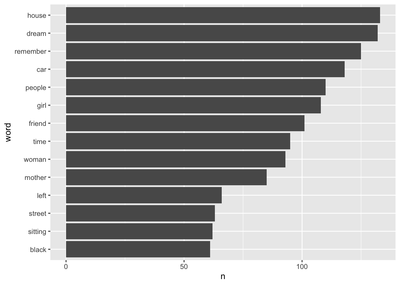
This gives us an overview of the most commonly used words in dreams recalled by all four samples. But it would be more interesting to see how the word use differs between the samples. However, we should be prepared for the possibility that the length of dreams may vary between samples. To control for this, we might want to convert our raw counts of words to proportions from the dream text. Let’s check for the variety of dream lengths by using str_count() function on our original dataset df - hence before we removed our stopwords. We will count the words in each dream and store the result in a vector called dream_lengths. The default for str_count is for the function to count characters if no pattern is given to match. However, if we pass it a second argument, specifying the regex for all sequences of non-space characters, it will count words instead. The regex includes the code for any non-white space character ‘\S’, with the addition of ‘+’ sign to indicate one or more non-white space characters, and the initial escape character ‘\’ as ‘\S’ is not recognised as an escape character without it.

dream_lengths <- str_count(df$dream, "\\S+")
plot(dream_lengths, xlab = "Dream Number")

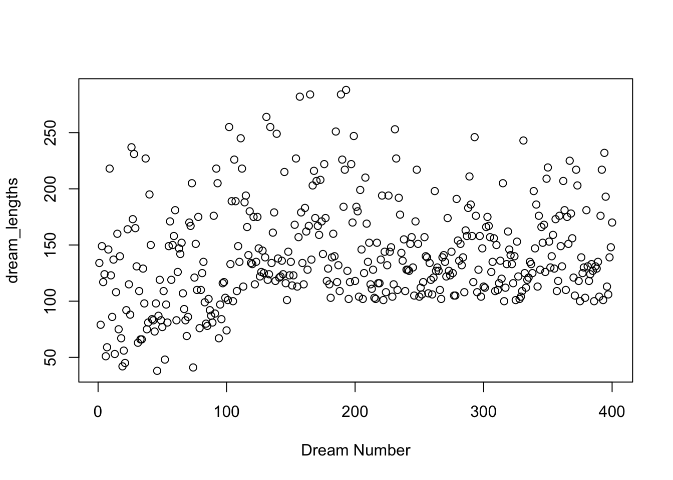
This is a good example of the use of the plot() function with a single vector in R. The default behaviour is to plot the values of the vector against the y-axis - dream_lengths in this case, and then use the index number (ie. the order in which each value occurs in the vector) as the x value. So our x-axis simple represents the order of the dreams, or as we have named this, the dream number. We can see here the range of dream lengths with the minimum being about 35 words and the maximum around 290 words. We could take the min, max, mean and SD if we wanted to be more specific.

min(dream_lengths); max(dream_lengths); mean(dream_lengths); sd(dream_lengths)

## [1] 38

## [1] 288

## [1] 141.0325

## [1] 45.09413

There is a great deal of variability in the dream lengths, so proportions will be better than raw counts to represent the frequency of each word.

Calculating word frequencies as proportions

We will want to count proportions after stopwords are removed. We have a choice here whether we want to express the frequency of individual words by proportion of a dream or proportion of a sample. These would have different interpretations. If the texts (in our case dreams) were much longer, proportion by text might be the better way to represent the data, but I suspect proportion by dream may not be very informative. Let’s try it and see what the results look like. We will group_by() dream_number so as to create proportion by dream. Then we use a summarise function to create a word count, and we use mutate to convert this to percentage. I used a second mutate to clean this up into two decimal places with the round() function. Finally, we use the tidyverse equivalent of sort() which is the arrange() function - but because we want this to be largest-to-smallest, we also include the desc() descending function.

df_word %>%
  group_by(dream_number, word) %>%
  summarise(n = n()) %>%
  mutate(percent = (n / sum(n))*100) %>%
  mutate(percent = round(percent, 2)) %>%
  arrange(desc(percent)) %>%
  ungroup

## `summarise()` has grouped output by 'dream_number'. You can override using the `.groups` argument.

## # A tibble: 15,500 × 4
##    dream_number word         n percent
##           <int> <chr>    <int>   <dbl>
##  1            6 remember     3    21.4
##  2          358 office       5    20  
##  3          355 dog          7    19.4
##  4          381 bus          6    18.2
##  5            2 hair         3    16.7
##  6           20 bed          3    16.7
##  7           83 store        5    16.7
##  8          260 car          6    16.7
##  9          399 test         6    15.8
## 10           13 dream        2    15.4
## # … with 15,490 more rows

So in dream number 6 the word ‘remember’ accounted for 21% of the non-stopwords used. That seems like a high proportion. It might be more useful to look at the data aggregated across samples. We can change the code to group_by sample instead of dream_number, then recalculate the most frequently occurring words as a proportion of words by sample.

df_word %>%
  group_by(sample, word) %>%
  summarise(n = n()) %>%
  mutate(percent = (n / sum(n))*100) %>%
  mutate(percent = round(percent, 2)) %>%
  arrange(desc(percent)) %>%
  ungroup()

## `summarise()` has grouped output by 'sample'. You can override using the `.groups` argument.

## # A tibble: 8,118 × 4
##    sample        word         n percent
##    <fct>         <chr>    <int>   <dbl>
##  1 college_women remember    55    1.63
##  2 hall_male     dream       57    1.31
##  3 hall_male     car         51    1.17
##  4 hall_male     house       49    1.13
##  5 vietnam_vet   woman       64    1   
##  6 hall_female   remember    40    0.96
##  7 college_women car         32    0.95
##  8 college_women dream       32    0.95
##  9 hall_female   dream       38    0.92
## 10 hall_female   house       36    0.87
## # … with 8,108 more rows

We can see that for the college women, the word ‘remember’ features the most frequently across the whole sample of 100 dreams and makes up roughly 1.6% of the non-stopwords in the dreams recorded.

Conclusion

We have explored how to tokenise texts, do some basic text cleaning and creating counts and proportions and finally graphed the simple word counts. In the next post in this series, I will explore the dream data using a clever technique from Julia Silge and David Robinson’s book that involves the spread() and gather() functions.