This is the third post in the series exploring text analytics with data from the dreambank.com. In the first post ‘Pulling text data from the internet’, I demonstrated how to use the rvest package to pull text data from the dreambank website. In the second post ‘Manipulating text data from dreams’ we saw how to turn the dream texts into a tidy format by unnesting the word tokens in each dream and running counts on the word frequencies. In this third post of the series, I am going to demonstrate some ways of comparing texts from Julia Silge and David Robinson’s book Text Mining with R - A tidy approach using the dream data set to illustrate the ideas, while also unpacking some of the steps a little further than in their book.

We will load our packages again and pull in the same data we analysed last time (see the previous post for details).

library(tidyverse)
library(tidytext)
library(stringr)
library(car)

The processing steps we used last time on the data was to add a dream number, unnest the tokens, remove stopwords, and then filter out underscores and digits.

df_word <- df %>%
  mutate(dream_number = row_number()) %>%
  unnest_tokens(word, dream) %>%
  anti_join(stop_words) %>%
  filter(str_detect(word, pattern = "_", negate = TRUE)) %>%
  filter(str_detect(word, pattern = '[\\d]', negate = TRUE))

Finally, we calculated word frequencies as proportions. This time we will store this as a new dataframe called df_proportion. Notice we have to remove the temporary ‘n’ variable. I am not sure why this is, but if you don’t deselect it, it seems to mess with the spread() function, creating multiple rows for the same word.

df_proportion <- df_word %>%
  group_by(sample, word) %>%
  summarise(n = n()) %>%
  mutate(percent = (n / sum(n))*100) %>%
  mutate(percent = round(percent, 2)) %>%
  select(-n) %>%
  arrange(desc(percent)) %>%
  ungroup()

Comparing word frequencies across samples

We might want to compare the frequencies across samples. We can use a technique that Juile Silge and David Robinson used to compare word frequencies across authors. This is a clever trick in which they use the spread() and gather() functions. Spread gives each sample their own column and makes the value proportion. Rather than do the spread and gather in one code chuck as in the book, I will do them as two separate stages to illustrate the process in more detail.

So let’s spread the data first. Think of this as taking the column of percentages/proportions and moving it into four separate columns: one for each sample. We are passing two arguments to the spread() function, the key (which contains the names of the items to form new columns) which is our ‘sample’ variable, and the value (what will the cells in each of these columns be filled with), which is the variable ‘percent’.

df_spread <- df_proportion %>%
  spread(sample, percent)

We could look at this new dataframe directly by clicking on the icon in the Global Environment, but you will notice lots of NA values. This is because each dream sample contains words that are unique to that sample and in a way these are the least informative - we can only make a binary comparison if one sample contains the word and the other does not. So we really want to see the variance in proportions for words that occur in more than one sample. To take a better look at these examples we can run our new dataframe called df_spread through a !is.na (is not NA) filter and then call the some() function from the car package. This is simply filtering out the rows in which the NA value occurs for the proportion of a word in any of our four samples.

df_spread %>%
  filter(!is.na(college_women) & !is.na(hall_female) & !is.na(hall_male) & !is.na(vietnam_vet)) %>%
  some()

## # A tibble: 10 × 5
##    word       college_women hall_female hall_male vietnam_vet
##    <chr>              <dbl>       <dbl>     <dbl>       <dbl>
##  1 arms                0.15        0.02      0.07        0.11
##  2 ball                0.12        0.02      0.09        0.02
##  3 care                0.03        0.1       0.02        0.05
##  4 completely          0.06        0.12      0.09        0.02
##  5 heavy               0.03        0.05      0.05        0.13
##  6 house               0.76        0.88      1.14        0.36
##  7 leaving             0.06        0.02      0.16        0.05
##  8 minutes             0.06        0.1       0.02        0.06
##  9 moving              0.03        0.02      0.02        0.05
## 10 running             0.12        0.02      0.3         0.06

Then the next step is to decide which sample is going to be our reference sample. This will have its column of frequencies replicated and stacked so that each of the other samples can be compared with it. When we gather(), we only include the samples to compare with the reference and not the reference itself. For simplicity, we can use the first column in our df (college_women) as our reference group and compare the other three samples to this. We might predict at this point that the hall_women will have the most similar dreams and then the hall_men, with the vietnam_vet being the most different. We can check this prediction later on when we run some correlation coefficients.

df_gather <- df_spread %>%
  gather(sample, proportion, hall_female:vietnam_vet)

We can take a quick look at the structure of the output, but we will filter out the NA values first, as we did for the df_spread dataset, as many are created for words that appear in one sample of dreams but not the other. Notice we do the same not-NA process (!is.na) on both the college_women data and the “proportion” variable. Remember that the college_women are our reference sample, so the ‘sample’ in this case tells us who provide the data in the proportion column.

df_gather %>%
  filter(!is.na(college_women) & !is.na(proportion))

## # A tibble: 1,950 × 4
##    word     college_women sample      proportion
##    <chr>            <dbl> <chr>            <dbl>
##  1 accident          0.03 hall_female       0.02
##  2 act               0.06 hall_female       0.05
##  3 afraid            0.24 hall_female       0.1 
##  4 age               0.61 hall_female       0.27
##  5 aged              0.09 hall_female       0.02
##  6 ages              0.03 hall_female       0.05
##  7 ago               0.12 hall_female       0.15
##  8 ahead             0.06 hall_female       0.02
##  9 air               0.15 hall_female       0.02
## 10 alarm             0.09 hall_female       0.02
## # … with 1,940 more rows

Next we can graph this data to inspect it more effectively. We use the df_gather as our data and set the aesthetics for x and y to proportion (which are our three samples) and college_women - which is our reference sample. As the college_women data will be used in all three graphs, it makes sense to assign it to the y axis, so we can scan down all three graphs vertically to make comparisons. There is another clever trick here with the colour variable. We will set it to the absolute value - abs() - of the difference between the college_women value and the other sample (proportion) value. This means that the darker the colour of the dot, the stronger the difference between the two proportion values. This allows us to use both shade (dark to light) and position away from the diagonal line as a measure of difference between samples. The paler the text the more similar the proportion use of the word in both samples.

library(scales)

ggplot(df_gather, aes(x = proportion, y = college_women,
                 colour = abs(college_women - proportion)))+
  geom_abline(colour = "gray40", lty = 2)+
  geom_jitter(alpha = 0.2, size = 2, width = 0.3, height = 0.3) +
  geom_text(aes(label = word), check_overlap = TRUE, vjust = 2)+
  scale_x_log10(labels = percent_format())+
  scale_y_log10(labels = percent_format())+
  scale_color_gradient(limits = c(0, 0.22),
                       low = "grey", high = "black")+
  facet_wrap(~sample, ncol = 1)+
  theme(legend.position = "none")+
  labs(y = "college_women", x = NULL)

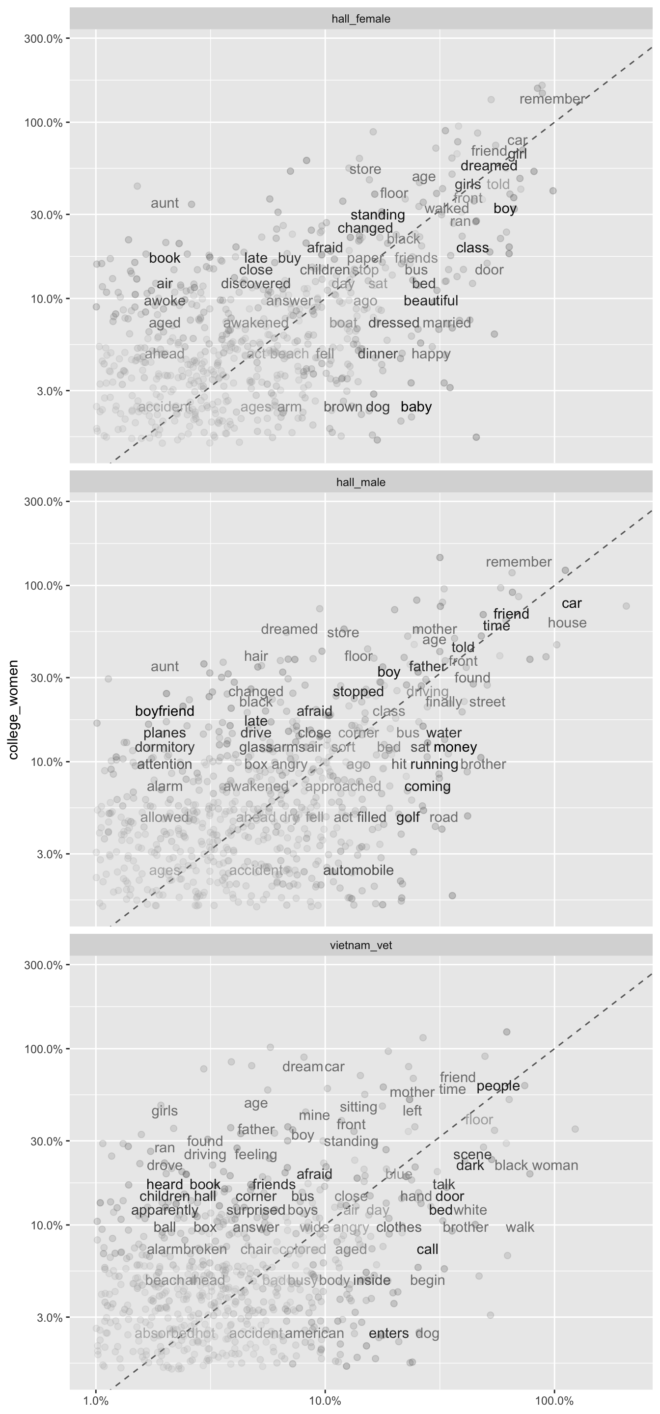
The words on or close to the line represent words that occurred at similar frequencies in both samples. As an example, we can see the word ‘remember’ occurred at high frequency in the first graph, in both the college_women and hall_female samples, as it is both high up and far to the right on the graph - but we can also observe that the closeness to the line suggests a similar frequency between the samples. In contrast, we can see on the same graph that the word “aunt” is quite far to the left of the line, indicating that it occurs more frequently in the college_women than the hall_women. This is also the case in the graph of college_women against hall_men, whereas this is not obvious in the final graph. It is possible that the word doesn’t occur at all in the vietnam_vet dream - therefore it would have been removed by graph function call. We can check the values for ‘aunt’ with a quick call of the df_spread data.frame (this is why it can be useful to keep both versions, rather than overwriting the data when we used the gather function).

df_spread %>%
  filter(word == "aunt")

## # A tibble: 1 × 5
##   word  college_women hall_female hall_male vietnam_vet
##   <chr>         <dbl>       <dbl>     <dbl>       <dbl>
## 1 aunt           0.43        0.02      0.02          NA

As we predicted, the lack of ‘aunt’ in the final graph was not due to a similar frequency between the samples, but rather the complete absence of the word in the vietnam_vet dreams. We can also see the size of difference between the frequency of the word in the college_women’s dreams and the other three samples is very large. Graphing the words in this way can give you a strong sense of these differences between the texts.

Correlation coefficient

We can use the base R function cor.test() to measure the degree of similarity between the proportions of words used in each sample. One approach is to prepare a new dataframe to carry out this test. Here we create a dataframe called df_cwhf(college_women and hall_female) and filter for just those rows that represent data for college women and hall_females. We can then run the cor.test() on this dataframe, by passing the variables ‘college_women’ and ‘proportion’ - the latter being just the proportion for the hall_female (because of the filter we applied).

df_cwhf <- df_gather %>%
  filter(sample == "hall_female")
cor.test(df_cwhf$college_women, df_cwhf$proportion)

## 
## 	Pearson's product-moment correlation
## 
## data:  df_cwhf$college_women and df_cwhf$proportion
## t = 34.676, df = 643, p-value < 2.2e-16
## alternative hypothesis: true correlation is not equal to 0
## 95 percent confidence interval:
##  0.7785169 0.8325231
## sample estimates:
##       cor 
## 0.8072027

Alternatively, we could use the syntax in Text mining with R, which subsets the data on the fly. We explicitly give a data argument, which is the df_gather dataframe, subsetted with samples == “hall_female”. We add a comma after this in the square brackets [ ], with no other argument, as we want to retain all the columns. Finally we provide our x and y values to be correlated in the formula format ~ x + y.

cor.test(data = df_gather[df_gather$sample == "hall_female", ], ~ proportion + college_women)

## 
## 	Pearson's product-moment correlation
## 
## data:  proportion and college_women
## t = 34.676, df = 643, p-value < 2.2e-16
## alternative hypothesis: true correlation is not equal to 0
## 95 percent confidence interval:
##  0.7785169 0.8325231
## sample estimates:
##       cor 
## 0.8072027

Let’s use this one-line technique to run the other two comparisons.

cor.test(data = df_gather[df_gather$sample == "hall_male", ], ~ proportion + college_women)

## 
## 	Pearson's product-moment correlation
## 
## data:  proportion and college_women
## t = 28.24, df = 648, p-value < 2.2e-16
## alternative hypothesis: true correlation is not equal to 0
## 95 percent confidence interval:
##  0.7062132 0.7753868
## sample estimates:
##       cor 
## 0.7427756

cor.test(data = df_gather[df_gather$sample == "vietnam_vet", ], ~ proportion + college_women)

## 
## 	Pearson's product-moment correlation
## 
## data:  proportion and college_women
## t = 12.03, df = 653, p-value < 2.2e-16
## alternative hypothesis: true correlation is not equal to 0
## 95 percent confidence interval:
##  0.3610922 0.4866471
## sample estimates:
##      cor 
## 0.425918

This reveals that all three samples correlate highly with the college_women, but the vietnam_vet dreams had a much lower correlation (.43) than the hall_female (.81) or the hall_male (.74). We could go on to use term frequency–inverse document frequency (tf-idf) to make a more complex comparison between the samples. In the next post, we will apply some of the sentiment analysis ideas from the book to the dream data. Let’s save our dataset df_word for next time.

save(df_word, file = "df_word.Rdata")